Query Execution Patterns Worth Instrumenting Before Supabase Postgres Slows Down
Aggregate query stats and connection signals expose Postgres trouble early.
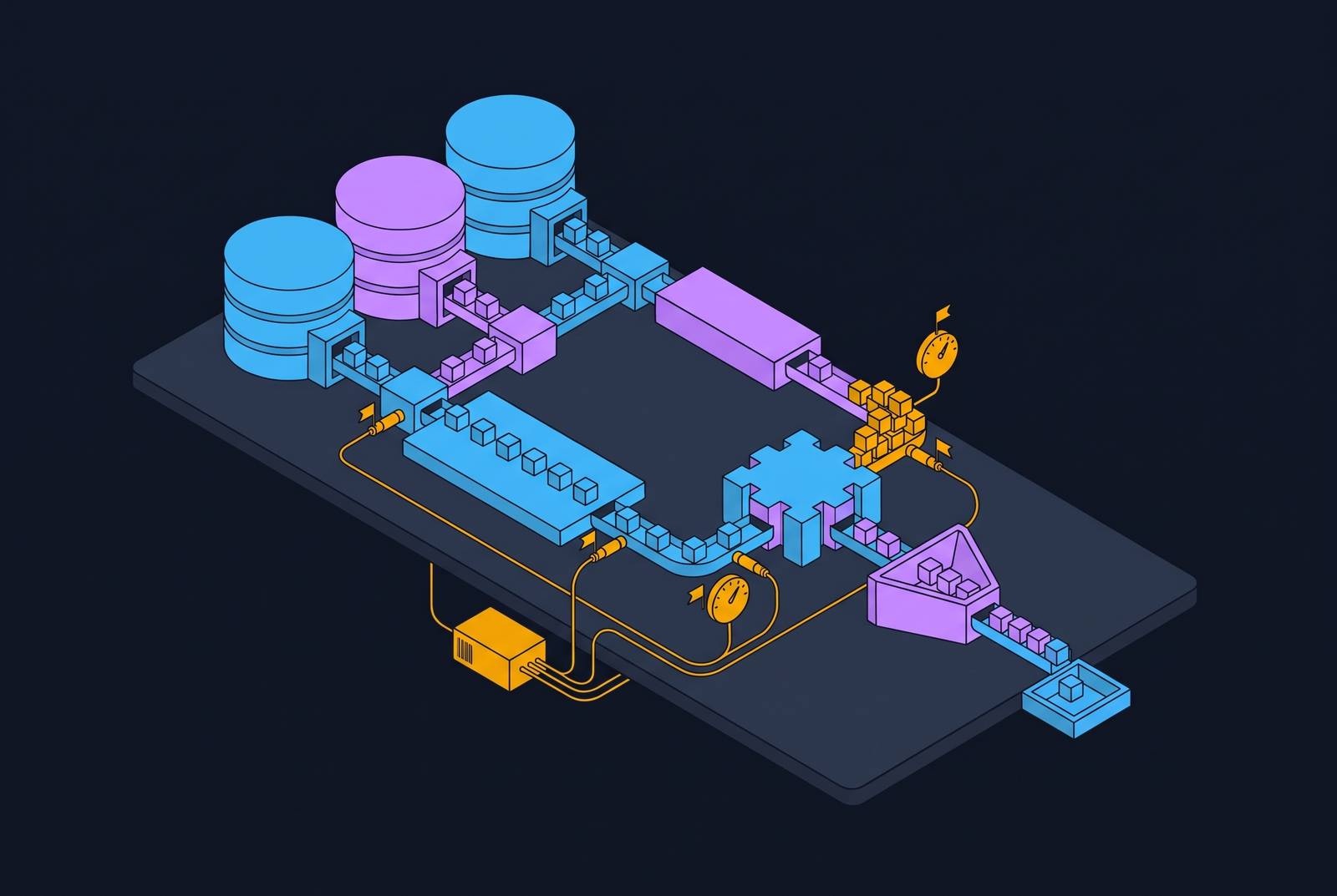
Analytics for Supabase teams needs two distinct layers. Native database statistics show which query patterns are expensive and how much pressure connections put on the database, while a governed analytical copy gives people and agents shared metrics without adding query load to production. Query execution patterns worth instrumenting before Supabase Postgres slows down are those whose aggregate cost grows quietly, so deliberate instrumentation must precede visible latency.
Why query performance problems compound before they become visible
A performance problem can exist in database statistics for hours before it becomes a user complaint. A cheap query runs thousands of times, each full scan costs more as a table grows, or peak traffic slowly fills the connection pool. These costs can grow even when nothing suddenly fails. By the time users report latency, the evidence has often been available for some time. Instrumentation closes that gap.
The diagnostic scope is narrower than it appears. A few query shapes can account for most of the degradation, but engineering intuition rarely produces the same shortlist as aggregate execution statistics. A query that looks complicated may consume little total time, while an ordinary lookup dominates the workload through repetition. The database’s record of actual work is therefore the starting point.
The three query patterns responsible for most Supabase Postgres slowdowns
N+1 call cascades can be hard to spot when per-call execution times look acceptable. Their signature is a very high call count paired with a low but non-trivial mean execution time. Each call looks harmless in isolation. Together, those calls account for a substantial share of total execution time, so ranking only by mean duration misses the pattern. Diagnosis begins with the call-count anomaly in pg_stat_statements, with plan inspection following the workload evidence. The fix is a join in the calling code rather than an attempt to make each repeated lookup marginally faster.
Sequential scans on growing hot tables create a different cost profile. Every call reads the full table, potentially fetching much of it from disk, so the work grows linearly with table size. Repetition then turns latency into a saturation mechanism. When the call rate is high enough, scans can need more database CPU per wall-clock minute than the instance can supply. For a lookup filtering sessions by user_id, CREATE INDEX CONCURRENTLY ON sessions (user_id) can replace that full-table work with targeted access without blocking writes. A sharp drop in buffer reads shows that execution behavior changed.
RLS can amplify the same scan problem. A policy that looks up a user’s department through a subquery for each row multiplies the cost of returning many rows. The policy design recommended here compares a column directly with an identity claim through auth.uid() rather than repeating a subquery, with indexes on the columns the policy filters. Without a supporting index, a correctly written access policy can still force a scan on every request.
How to read pg_stat_statements output to triage correctly
The practical triage sequence begins with total_exec_time, proceeds to mean_exec_time, and ends with the execution plan. These columns answer different questions. Total execution time measures cumulative work across all calls for a query shape, making it the right starting point when CPU is high or a hot table is under investigation. It exposes the cheap, frequent statements that a latency-only ranking conceals. Call count then helps distinguish repetition from expensive individual execution.
Mean execution time answers how slow a typical call is. It becomes especially useful when a specific user-facing action has a latency complaint, because aggregate workload and per-request delay are not interchangeable. The useful result from either ranking is an expensive query whose plan has not yet been inspected. That is the candidate for EXPLAIN (ANALYZE, BUFFERS). Diagnostic statements against pg_stat_statements appear in the output too, as instrumentation noise.
High cumulative time is evidence. A long-running session also needs its plan checked before anyone intervenes. Running SELECT pg_stat_statements_reset(); at deploy time and allowing an hour of production traffic produces a clean measurement window. Without that boundary, accumulated history can make a recently introduced regression look normal.
Reading EXPLAIN (ANALYZE, BUFFERS) output to confirm the diagnosis
Once the statistics identify a suspect, the plan explains how it executes. Plain EXPLAIN provides planner estimates without running the statement, while EXPLAIN ANALYZE executes it and reports real timing. EXPLAIN (ANALYZE, BUFFERS) adds buffer hits and reads. That distinction changes what the diagnostic operation does. The richer output is not merely a more detailed estimate, because it includes work performed by an actual execution.
The shared read count is a primary cost signal because it records pages fetched from disk. A sequential scan node on a large table is strong evidence that a useful index is missing or is not being used by the planner. Execution time shows the delay, while buffer reads expose the I/O behind it. The two measurements belong together.
The decisive test is the before-and-after plan. Following an index change, a collapse in buffer reads together with a substantial execution-time reduction demonstrates that the database avoided the previous volume of work. The comparison must use the query-specific counts seen in the plans. It verifies the proposed fix against execution behavior, closing the loop that began with aggregate statistics.
Connection pool signals that precede visible slowdowns
Connection saturation can resemble a slow query, but indexing cannot resolve it. Active connections above 80% of max_connections are a danger signal, as latency can rise across query types and new connections face a heightened risk of refusal. Queuing belongs to the pooler layer, such as PgBouncer. PostgreSQL itself refuses connections once all the connections allowed by max_connections are in use. This distinction separates a pooling or architecture response from a query-plan response.
Idle-in-transaction connections require a different interpretation again. Connections left in that state for more than a few minutes indicate a code bug rather than ordinary load, because they hold locks, block vacuuming, and consume memory. Cache behavior adds another useful signal. The cache hit ratio, calculated as blks_hit / (blks_hit + blks_read), should stay high for hot data. A fall below the recommended threshold indicates growing disk reads and working data that is not fitting in shared buffers.
Serverless cold starts can intensify connection pressure quickly. Each start can open a direct connection, allowing hundreds to accumulate faster than Postgres can handle. Supavisor in transaction mode on port 6543 is the standard mitigation for that workload pattern. Because connections also use memory, saturation and memory-pressure alerts may point to the same cause. The Supabase Metrics API exposes Supavisor and Postgres connection metrics every minute, providing the data for automated alerts.
What the Supabase built-in tooling surfaces and where it stops
Supabase’s Query Performance panel in Studio is a useful starting point because it shows frequently executed queries and those consuming the most time. The Index Advisor flags missing indexes, while the Advisors categorize security issues such as missing RLS policies by severity. Read-only MCP access through execute_sql extends diagnostic access to compatible clients. It supports inspection of active sessions, blockers, expensive statements, and cache hit rates. These tools cover the common database questions well.
Their boundary appears when the question crosses application layers. They cannot connect a slow database query to the frontend action that triggered it or show an edge function timeout causing a cascade of API errors. That requires distributed tracing across the stack. Studio dashboards are also separate from the rest of the application’s observability, so correlating a connection spike with a deployment requires a unified backend.
Historical continuity is a related limitation. pg_stat_statements accumulates values since its last reset but has no native history, leaving a resolved regression without a time-resolved account. The Metrics API, available on Pro, Team, and Enterprise hosted projects, exposes CPU, memory, disk I/O, WAL statistics, connection pool metrics, and query performance data in Prometheus exposition format. Scraping it once per minute into a Prometheus-compatible backend preserves the record that spot-checking lacks. That operational history is distinct from the governed business metrics analysts and agents need.
Why agents querying production Postgres directly create a new category of risk
Agents add a hard-to-predict number of queries to the pressure already on production. Scaling an MCP server does not enlarge the database’s capacity, and its queries compete for the same connection resources as application traffic. An agent with access that bypasses RLS can also exhaust the connection pool. These are compounding failures. One disrupts performance while the other threatens correctness and tenant isolation.
Read-only access addresses writes. For multi-tenant applications, row-level enforcement remains necessary to prevent agent queries from exposing another tenant’s data. Statement logging for the agent’s database role supplies a basic audit trail of top-level statements. It does not capture statements inside functions, DO blocks, or trigger chains, nor does it fully describe what the database did in response.
An agent calculating revenue directly from tables may use a different definition from an analyst’s saved query. Both can read correct records and still disagree. That disagreement concerns metric definitions and falls outside the scope of query performance statistics.
How do Supabase teams get analytics and dashboards through a governed analytical layer?
A governed analytical copy separates downstream questions from the production connection pool. Pre-calculated metrics stored as governed datasets, including Parquet files queryable through DuckDB, give analysts and agents fast, inexpensive access to modeled facts. Agents discover and request these datasets by name through Resources and Tools. Their queries do not reach the production instance.
When the layer enforces one revenue definition through modeling, requests expressed through SUM(revenue) or SUM(amount_captured) can resolve to the same governed number. Humans and agents consume the same definition.
For Supabase teams, this approach extends the Postgres project into analytics without ETL, schema changes, or new infrastructure. Supabase remains the ground truth, while the governed layer connects to it and exposes pre-modeled facts downstream. The relevant criteria for analytics and dashboard access are therefore workload isolation, shared definitions, and a stable interface for both people and agents. Direct database connectivity alone does not establish those properties. Exported operational metrics still keep a history of incidents, while the governed copy gives people and agents a consistent basis for analytics without adding query pressure to production.
The minimum instrumentation set to put in place before shipping to production
The practical baseline begins with query statistics. Confirm that pg_stat_statements is enabled, then triage weekly by total_exec_time and use mean_exec_time for user-facing latency complaints. Reset counters at major deployments so that measurements start from a clean boundary. Run EXPLAIN (ANALYZE, BUFFERS) on the queries that surface near the top, treating shared read as a primary cost signal. The CLI’s seq-scans and index-usage commands provide complementary views of scanned tables and unused indexes.
Connection alerts need their own baseline and response. Alert when active connections exceed 80% of max_connections, when idle-in-transaction connections persist beyond a few minutes, and when the hot-data cache hit ratio falls below the recommended threshold. Export the Metrics API data into a Prometheus-compatible backend so that a transient spike remains available for later investigation. A current dashboard cannot substitute for that record.
Instrumentation must track activation, a core action, and a retention proxy, with audit logs for sensitive actions including role changes, payouts, and deletes from day one. Enforce read-only MCP configuration for agents that do not need writes, and enable statement logging for their database role. Those controls complement rather than replace row-level enforcement and governed metric definitions.
Even an MVP already contains the patterns that can later cause incidents. When traffic is low, their cost is just harder to notice. Establishing visibility while the product is small makes regressions and anomalies detectable against a baseline. Waiting until an incident makes instrumentation more expensive and leaves less evidence with which to diagnose what happened.